Dimension tables: efficiently adding details of processes and flows

In the Quickstart tutorial we saw how to draw some simple Sankey diagrams and partition them in different ways, such as this:

But to do the grouping on the right-hand side we had to explicitly list which people were “Men” and which were “Women”, using a partition like this:

customers_by_gender = Partition.Simple('process', [
    ('Men', ['Fred', 'James']),
    ('Women', ['Susan', 'Mary']),
])

We can show this type of information more efficiently – and with less code – by using dimension tables.

Dimension tables

The table we’ve seen before is a flow fact table – it lists basic information about each flow:

• source: where the flow comes from

• target: where the flow goes to

• type or material: what is flowing

• value: the size (in tonnes, GJ, £ etc) of the flow

An example of this type of table is shown at the top right of this diagram:

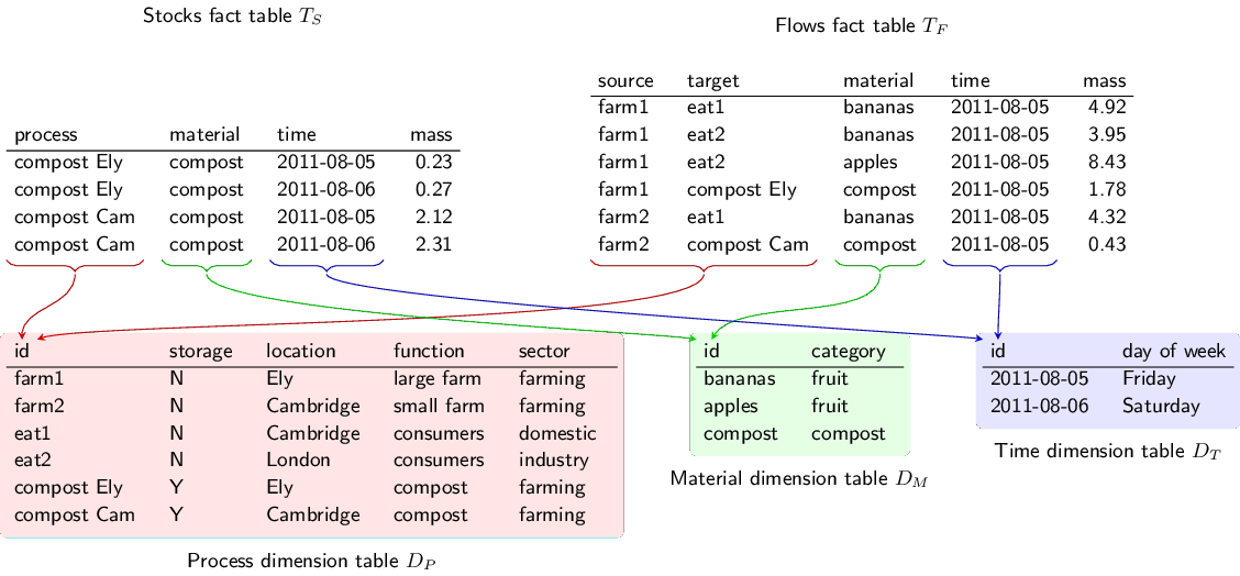
The dimension tables add extra information about the source/target and type of the flows (the diagram above also shows extra information about the time period the flow relates to, but we’re not worrying about time in this tutorial). For example, “farm2” has a location attribute set to “Cambridge”.

This tutorial will show how to use dimension tables in floweaver.

# Load the same data used in the quickstart tutorial
import pandas as pd
flows = pd.read_csv('simple_fruit_sales.csv')
flows

	source	target	type	value
0	farm1	Mary	apples	5
1	farm1	James	apples	3
2	farm2	Fred	apples	10
3	farm2	Fred	bananas	10
4	farm2	Susan	bananas	5
5	farm3	Susan	apples	10
6	farm4	Susan	bananas	1
7	farm5	Susan	bananas	1
8	farm6	Susan	bananas	1

# Load another table giving extra information about the
# farms and customers. `index_col` says the first column
# can be used to lookup rows.
processes = pd.read_csv('simple_fruit_sales_processes.csv',
                        index_col=0)
processes

	type	location	organic	sex
id
farm1	farm	Barton	yes	NaN
farm2	farm	Barton	yes	NaN
farm3	farm	Ely	no	NaN
farm4	farm	Ely	yes	NaN
farm5	farm	Duxford	no	NaN
farm6	farm	Milton	yes	NaN
Mary	customer	Cambridge	NaN	Women
James	customer	Milton	NaN	Men
Fred	customer	Cambridge	NaN	Women
Susan	customer	Cambridge	NaN	Men

Each id in this table matches a source or target in the flows table above. We can use this extra information to build the Sankey.

# Setup
from floweaver import *

# Set the default size to fit the documentation better.
size = dict(width=570, height=300)

Because we now have two tables (before we only had one so didn’t have to worry) we must put them together into a Dataset:

dataset = Dataset(flows, dim_process=processes)

Now we can use the type column in the process table to more easily pick out the relevant processes:

nodes = {
    'farms': ProcessGroup('type == "farm"'),
    'customers': ProcessGroup('type == "customer"'),
}

Compare this to how the same thing was written in the Quickstart:

nodes = {
    'farms': ProcessGroup(['farm1', 'farm2', 'farm3',
                           'farm4', 'farm5', 'farm6']),
    'customers': ProcessGroup(['James', 'Mary', 'Fred', 'Susan']),
}

Because we already know from the process dimension table that James, Mary, Fred and Susan are “customers”, we don’t have to list them all by name in the ProcessGroup definition – we can write the query type == "customer" instead.

Note

See the API Documentation for floweaver.ProcessGroup for more details.

The rest of the Sankey diagram definition is the same as before:

ordering = [
    ['farms'],       # put "farms" on the left...
    ['customers'],   # ... and "customers" on the right.
]
bundles = [
    Bundle('farms', 'customers'),
]
sdd = SankeyDefinition(nodes, bundles, ordering)
weave(sdd, dataset).to_widget(**size)

Again, we need to set the partition on the ProcessGroups to see something interesting. Here again, we can use the process dimension table to make this easier:

# Create a Partition which splits based on the `sex` column
# of the dimension table
customers_by_gender = Partition.Simple('process.sex',
                                       ['Men', 'Women'])

nodes['customers'].partition = customers_by_gender
weave(sdd, dataset).to_widget(**size)

For reference, this is what we wrote before in the Quickstart:

customers_by_gender = Partition.Simple('process', [
    ('Men', ['Fred', 'James']),
    ('Women', ['Susan', 'Mary']),
])

And we can use other columns of the dimension table to set other partitions:

farms_by_organic = Partition.Simple('process.organic', ['yes', 'no'])

nodes['farms'].partition = farms_by_organic
weave(sdd, dataset).to_widget(**size)

Finally, a tip for doing quick exploration of the data with partitions: you can automatically get a Partition which includes all the values that actually occur in your dataset using the dataset.partition method:

# This is the logical thing to write but
# it doesn't actually work at the moment :(
# nodes['farms'].partition = dataset.partition('process.organic')

# It works with 'source.organic'... we can explain later
nodes['farms'].partition = dataset.partition('source.organic')

# This should be the same as before
weave(sdd, dataset).to_widget(**size)

Summary

The process dimension table adds extra information about each process. You can use this extra information to:

1. Pick out the processes you want to include in a ProcessGroup (selection); and

2. Split apart groups of processes based on different attributes (partitions).

Things to try:

• Make a diagram showing the locations of farms on the left and the locations of customers on the right